Recently I have completed professor Andrew Ng’s Coursera class on Machine Learning. I learnt a lot from this and I liked the most the practical exercises. The course covers general methods of machine learning, starting with linear regression, logistic regression, neural networks, clustering and many others. You can find praises for this class basically everywhere online so I won’t say any more here.

Since I’m not a practitioner of Machine Learning techniques, at the end of the class I wanted to find an aproachable and interesting project to practice somehow my newly acquired knowledge. So I stumbled upon the amazing work of Julia Evans.

In this blog I’ve followed and build upon that, and convinced an already trained (by Google!) Neural Network that my cat is actually a penguin, or a mouse or other different animals (Hint: It actually works!) I’ve removed many details and added more comments throughout the code. Please check her original blog post to better understand what’s happening at every point.

If you want to follow along, check her installation instructions to configure a Docker container with all the necessary libraries in it. Also here’s my Jupyter Notebook. While doing the Docker setup part I had a few issues, but nothing that couldn’t be solved with a few Google searches.

The trickiest one was that the backpropagation method returned a matrix with all zeros. The bottom line is that by default Caffe does not backpropagate to the data since it has no parameters. You need to force this by adding a parameter to your model. More details here.

Part 1 - Setup

This is completely coverd in the Julia Evans’ referenced article and you can find it in my Jupyter Notebook as well. Basically we need to do few things before we can start playing with the neural network:

• Prepare the necessary libraries: Caffe, Pandas, mathplotlib, numpy, etc.
• Load the labels of the neural network
• Load the model already trained on a huge set of animal images
• Define some auxiliary functions to get images from URLs and convert them to PNG
• Create the prediction function

Part 2 - Testing the Neural Network

We’re going to test the network first. A Persian cat is detected in the image below, with probability 13.94%. Sounds (about) right. More on this later.

img_url = 'https://github.com/livz/livz.github.io/raw/master/assets/images/liz.jpg'
img_data = get_png_image(img_url)

probs = predict(img_data, n_preds=1)

label: 283 (Persian cat)
certainty: 13.94%

Part 3 - Breaking the predictions

Step 1 - Calculate the gradient

First we’ll calculate the gradient of the neural network. The gradient is the derivative of the network. The intuition behind this is that the gradient represents the direction to take to make the image look like something. So we’ll calculate the gradient to make the cat look like a mouse for example.

def compute_gradient(image_data, intended_outcome):
    predict(image_data, display_output=False)
    
    # Get an empty set of probabilities
    probs = np.zeros_like(net.blobs['prob'].data)
    
    # Set the probability for our intended outcome to 1
    probs[0][intended_outcome] = 1
    
    # Do backpropagation to calculate the gradient for that outcome
    gradient = net.backward(prob=probs)
    
    return gradient['data'].copy()

mouse = 673        # Line 674 in synset_words.txt
grad = compute_gradient(img_data, mouse)    

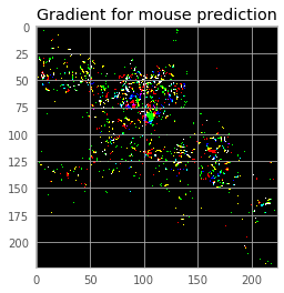
Very important, because the gradient is the same shape as the the original image, we can display it as an image!. But we need to scale it up, otherwise it won’t be visible, since the order of magniture of gradient is e-08. So let’s display the gradient for the prediction above:

# Display scaled gradient
display(grad / np.percentile(grad, 98))

plt.title('Gradient for mouse prediction')

Step 2: Find the direction towards a different prediction

We’ve already calculated gradient via compute_gradient() function, and drawn it as a picture. In this step we want to create a delta which emphasizes the pixels in the picture that the neural network thinks are important.

Below we can play with different values and add or substract small multiples of delta from our image and see how the predictions change. The modified image is then displayed. Notice how the pixels are slightly affected.

delta = np.sign(grad)
multiplicator = 0.9
new_predictions = predict(np.round(img_data + multiplicator*delta), n_preds=5)

label: 673 (mouse, computer mouse), certainty: 52.87%
label: 508 (computer keyboard, keypad), certainty: 12.23%
label: 230 (Shetland sheepdog, Shetland sheep dog), certainty: 4.22%
label: 534 (dishwasher, dish washer), certainty: 2.73%
label: 742 (printer), certainty: 2.6%

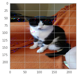
We’ve added a very light version of the gradient to the original image. This increased the probability of the label we used to compute the gradient - mouse, which now has 52.87% probability. Not bad at all but the image is visibly altered. Let’s see if we can do better.

So insted of adding delta multiplied by a big number (0.9), we’ll work in smaller steps, compute the gradient towards our desired outcome at each step and each time modify the image slightly.

Step 3 - Loop to find the best values

Slowly go towards a different prediction. At each step compute the gradient for our desired label, and make a slight update of the image. The following steps compute the gradiend of the image updated at previous step then update it slightly.

The most interesting function of this whole session is below. Spend a few minutes on it!

def trick(image, desired_label, n_steps=10):
    # Maintain a list of outputs at each step
    # Will be usefl later to plot the evolution of labels at each step.
    prediction_steps = []
    
    for _ in range(n_steps - 1):
        preds = predict(image, display_output=False)
        prediction_steps.append(np.copy(preds))
        grad = compute_gradient(image, desired_label)
        delta = np.sign(grad)
        # If there are n steps, we make them size 1/n -- small!
        image = image + delta * 0.9 / n_steps
    return image, prediction_steps

Part 4 - Final results

Transform the cat into a penguin (or mouse)

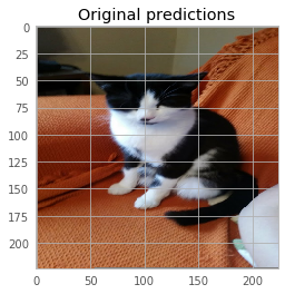
… without affecting the apparence of the image. First let’s check the original predictions, to see what is our starting point:

# Check Original predictions
pred  = predict(img_data, n_preds=5)
plt.title("Original predictions")

label: 283 (Persian cat), certainty: 13.94%
label: 700 (paper towel), certainty: 13.38%
label: 673 (mouse, computer mouse), certainty: 6.05%
label: 478 (carton), certainty: 5.66%
label: 508 (computer keyboard, keypad), certainty: 4.7%

Now let’s trick the Neural Network:

mouse_label = 673
penguin_label = 145
new_image, steps = trick(img_data, penguin_label, n_steps=30)

preds = predict(new_image)
plt.title("New predictions for altered image")

label: 145 (king penguin, Aptenodytes patagonica), certainty: 51.84%
label: 678 (neck brace), certainty: 4.76%
label: 018 (magpie), certainty: 4.27%
label: 667 (mortarboard), certainty: 3.02%
label: 013 (junco, snowbird), certainty: 2.52%
label: 148 (killer whale, killer), certainty: 2.04%

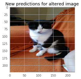
It still looks like a cat, with no visible differences compared to the intial picture. But after only 10 iterations, the cat can become a mouse with 96.72% probability, or a king penguin actually with a probability of 51.84% after 30. We can do a lot better with more iterations but it takes more time. Notice there is no visible change in the image pixels!

Plot the evolution of predictions

Another cool thing to do is plot the evolution of predictions for a few chosen labels and see what happens with the probabilities at every small step:

# Plot evolution of different labels at each step
def plot_steps(steps, label_list, **args):
    d = {}
    for label in label_list:
        d[get_label_name(label)] = [s[0][label] for s in steps]
    df = pd.DataFrame(d)
    df.plot(**args)
    plt.xlabel('Step number')
    plt.ylabel('Probability of label')

mouse_label = 673
keyboard_label = 508
persian_cat_label = 283
penguin_label = 145

label_list = [mouse_label, keyboard_label, persian_cat_label, penguin_label]
plot_steps(steps, label_list, figsize=(10, 5))
plt.title("Prediction for labels at each step")

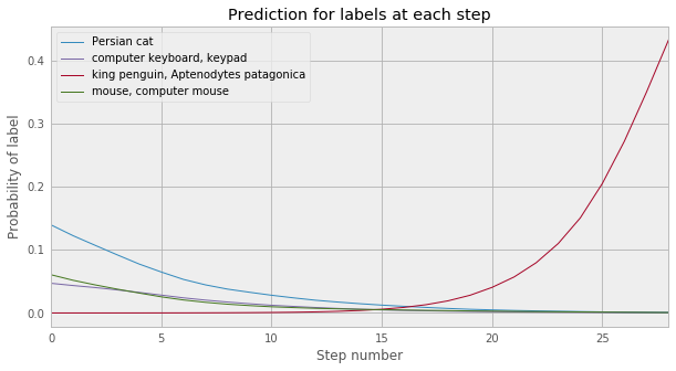
Morphing the cat

Initially the first prediction was Persian cat (label 283) with 13.94% certainty. Although the image was correctly recognised as a cat, the probability is really not that great. Let’s try to obtain a better score and address all the doubts that there is a Persian cat in the picture (It actually isn’t! A Persian cat looks massively different).

persian_cat_label = 283
cat_persian, steps = trick(img_data, persian_cat_label, n_steps=10)
preds = predict(cat_persian)
plt.title("Persian or not?")

label: 283 (Persian cat), certainty: 99.9%
label: 332 (Angora, Angora rabbit), certainty: 0.03%
label: 281 (tabby, tabby cat), certainty: 0.01%
label: 259 (Pomeranian), certainty: 0.01%
label: 700 (paper towel), certainty: 0.01%
label: 478 (carton), certainty: 0.0%

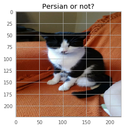
After just 10 iterations, we managed to grow the confidence of the predicted label **from 13.94% to 99.9% certainty**!

Conclusions

After going through the pain of setting up the correct libraries and train them, Neural networks actually can be very fun! If you’re interested, the Coursera class is definitely a strong place to start, and plenty of resources online and ways to continue your journey into ML afterwards!